42 pivot table 2 row labels
How to rename group or row labels in Excel PivotTable? To rename Row Labels, you need to go to the Active Field textbox. 1. Click at the PivotTable, then click Analyze tab and go to the Active Field textbox. 2. Now in the Active Field textbox, the active field name is displayed, you can change it in the textbox. Pivot table row labels side by side - Excel Tutorials You can copy the following table and paste it into your worksheet as Match Destination Formatting. Now, let's create a pivot table ( Insert >> Tables >> Pivot Table) and check all the values in Pivot Table Fields. Fields should look like this. Right-click inside a pivot table and choose PivotTable Options…. Check data as shown on the image below.
How to Add Two-Tier Row Labels to the Pivot Table in Google Sheets Step 1: Click on any cell in the Pivot Table so that the Pivot table editor sidebar appears on the right side of Google Sheets. Pivot Table, with Pivot table editor sidebar visible. As you can see, the item column is used as the row labels or headers in the Pivot table.

Pivot table 2 row labels
Pivot Table adding "2" to value in answer set 1) Right click your pivot table -> Pivot table options -> Data -> Change "Number of items to retain per field" to NONE 2) Wipe all rows in your data source except for the headers 3) Refresh the pivot table 4) Save, and close all instances of Excel 5) Reopen the file, and paste your data 6) Refresh the pivot table Ranking to a Pivot Table with multiple Row Labels I have a pivot table with multiple Row Labels: Team and Player. I created a second Pts column and used 'Show Values As - Rank Largest to Smallest', but it's not working. It's showing up as '1' for all columns, regardless of whether or not I pick 'Team' or 'Player' as the base field. If I remove 'Team' as a Row Label, however, it works perfectly. How to add side by side rows in excel pivot table - AnswerTabs To display more pivot table rows side by side, you need to turn on the Classic PivotTable layout and modify Field settings. For example will be used the following table: You have to right-click on pivot table and choose the PivotTable options. Then swich to Display tab and turn on Classic PivotTable layout:
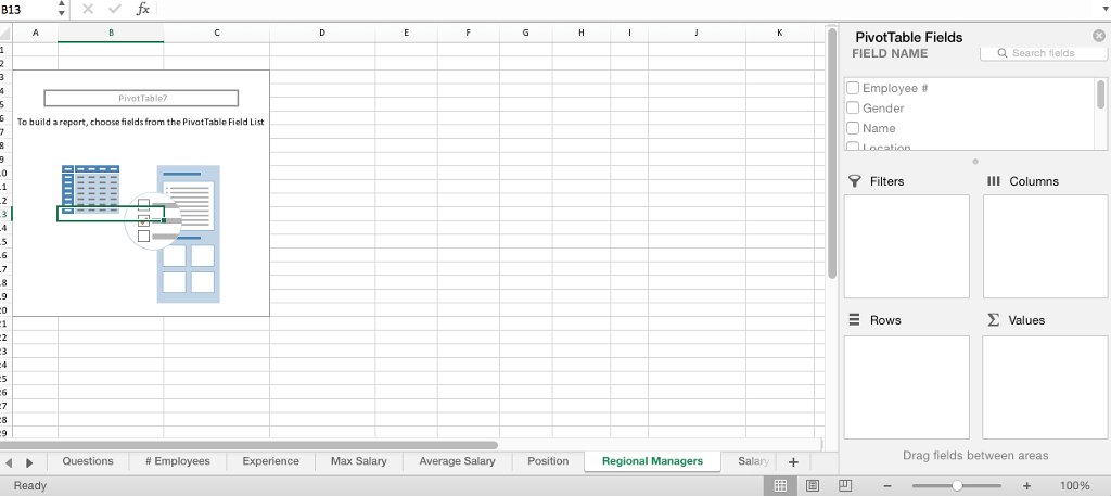
Pivot table 2 row labels. pivot table how to combine 2 row labels - MrExcel Message Board Excel Questions pivot table how to combine 2 row labels sdsurzh Nov 6, 2013 S sdsurzh Board Regular Joined Sep 27, 2009 Messages 248 Nov 6, 2013 #1 Hi, i am having the pivot table in the below format. my concern is how i can combine both A & AA together the source is from data connection and not from the excel. How to Customize Your Excel Pivot Chart Data Labels The Data Labels command on the Design tab's Add Chart Element menu in Excel allows you to label data markers with values from your pivot table. When you click the command button, Excel displays a menu with commands corresponding to locations for the data labels: None, Center, Left, Right, Above, and Below. None signifies that no data labels ... Pivot table row labels in separate columns • AuditExcel.co.za Our preference is rather that the pivot tables are shown in tabular form (all columns separated and next to each other). You can do this by changing the report format. So when you click in the Pivot Table and click on the DESIGN tab one of the options is the Report Layout. Click on this and change it to Tabular form. How to Add Rows to a Pivot Table: 9 Steps (with Pictures) 2 Click any cell in the PivotTable. This opens the PivotTable Fields panel on the right side of Excel. If you have already moved the appropriate field to the Rows area but don't see a row that's in your source data, just press Alt + F5 or right-click the pivot table and select Refresh. 3 Drag a field into the "Rows" area on PivotTable Fields.
Pivot Table "Row Labels" Header Frustration - Microsoft Tech Community Public Sector. Internet of Things (IoT) Azure Partner Community. Expand your Azure partner-to-partner network. Microsoft Tech Talks. Bringing IT Pros together through In-Person & Virtual events. MVP Award Program. Find out more about the Microsoft MVP Award Program. get a row label from pivot table - Microsoft Tech Community Creating PivotTable add data to data model by checking Create PivotTable and after that convert it to cube formulas. Now you may take these formulas and convert it to form you need, for example in H3 it could be =CUBEVALUE( "ThisWorkbookDataModel", CUBEMEMBER("ThisWorkbookDataModel", " [Measures]. Duplicate Items Appear in Pivot Table - Excel Pivot Tables In Row 2 of the new column, enter the formula =TRIM(C2). Copy the formula down to the last row of data in the source table. If the source data is stored in an Excel Table, the formula should copy down automatically. Refresh the pivot table ; Remove the City field from the pivot table, and add the CityName field to replace it. _____ How to Use Excel Pivot Table Label Filters To change the Pivot Table option, and allow multiple filters, follow these steps: Right-click a cell in the pivot table, and click PivotTable Options. In the PivotTable Options dialog box, click the Totals & Filters tab In the Filters section, add a check mark to 'Allow multiple filters per field.'
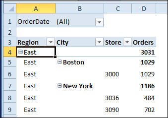
Pivot Table Row Labels In the Same Line - Beat Excel! Then navigate to "Layout & Print" tab and click on "Show item in tabular form" option. Do this procedure also for "Dealer" field and your table will look like this: If you also want dealer names to repeat on each row, reopen "Dealer field settings and check "Repear item labels" option in "Layout & Print" tab. excel - Custom row labels in PivotTable - Stack Overflow you can give nicknames to the fields that you are checking which populate the pivot table. If you go the pivot table data and right click you can change the value field settings to give a custom name to a row/series but I do not know about individual data points. path: pivot table data => right click => select Field Settings => edit custom name. Multi-level Pivot Table in Excel (In Easy Steps) First, insert a pivot table. Next, drag the following fields to the different areas. 1. Category field and Country field to the Rows area. 2. Amount field to the Values area. Below you can find the multi-level pivot table. Multiple Value Fields First, insert a pivot table. Next, drag the following fields to the different areas. 1. Combining two+ Columns to form one Row label column in Pivot Table Hello, I have multiple sets of data that occur in 2 column increments. The first column is a list of part numbers, the second is their value for that month. I want a pivot table that combines all of the first columns into one master row label of Part numbers and then the values will be listed out in each subsequent column. If a particular month doesn't have a part number in its data, then it ...
How to Show the Percentage of Row Total in the Pivot Table - MS Excel | Excel In Excel
Design the layout and format of a PivotTable Right-click the field name and then select the appropriate command — Add to Report Filter, Add to Column Label, Add to Row Label, or Add to Values — to place the field in a specific area of the layout section. Click and hold a field name, and then drag the field between the field section and an area in the layout section.

Pivot table row labels side by side
Sorting to your Pivot table row labels in custom order [quick tip] Create a pivot table with data set including sort order column. Add sort order column along with classification to the pivot table row labels area. Add the usual stuff to values area. Set up pivot table in tabular layout. Remove sub totals; Finally hide the column containing sort order. Your new pivot report is ready.
Help Online - Origin Help - Pivot Table
How to make row labels on same line in pivot table? Make row labels on same line with PivotTable Options You can also go to the PivotTable Options dialog box to set an option to finish this operation. 1. Click any one cell in the pivot table, and right click to choose PivotTable Options, see screenshot: 2.
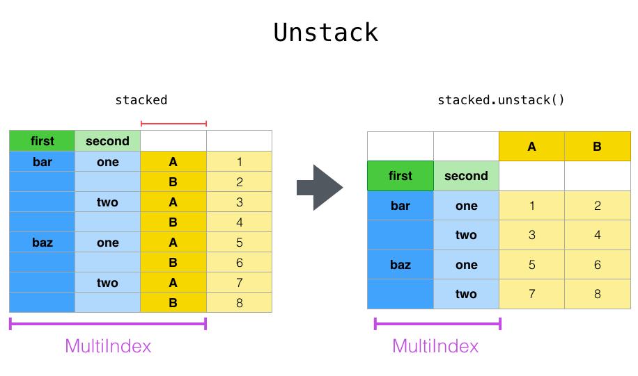
Reshaping and pivot tables — pandas 1.1.4 documentation
Pivot Table Multiple Row Labels? [SOLVED] You can, of course, create a pivot table that sums the values just at the owner level. then, create a second pivot table that sums the values at the Engineer level. If you need to present this data in a contiguous table, you can create a new Excel table and reference to the pivot table values with formulas (=PivotTableSheet!A1) cheers Microsoft MVP
How to Setup Source Data for Pivot Tables - Unpivot in Excel
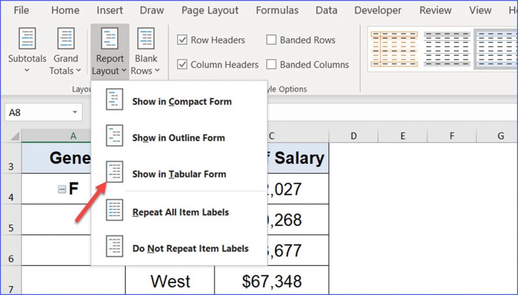
Pivot Table Row Labels - Microsoft Community If you go to PivotTable Tools > Analyze > Layout > Report Layout > Show in Tabular Form, your column headers will be used for the row labels. Every once in a while there's a sudden gust of gravity... Report abuse 1 person found this reply helpful · Was this reply helpful? Yes No A. User Replied on December 19, 2017

How to Sort Pivot Table Row Labels, Column Field Labels and Data Values with Excel VBA Macro ...
Repeat item labels in a PivotTable - support.microsoft.com Right-click the row or column label you want to repeat, and click Field Settings. Click the Layout & Print tab, and check the Repeat item labels box. Make sure Show item labels in tabular form is selected. Notes: When you edit any of the repeated labels, the changes you make are applied to all other cells with the same label.

Can't apply value filter to excel pivot table without affecting subtotals - Subtotal filtered ...
Shifting Row Sub label to another column in Pivot Table 37 6. If you are OK with having the country in Column 2, merely change the Report Layout to show in tabular form and you may also want to do not show subtotals. - Ron Rosenfeld. Oct 25, 2021 at 13:44. Add a comment.
33 Pivot Table Blank Row Label - Labels Database 2020
How to add side by side rows in excel pivot table - AnswerTabs To display more pivot table rows side by side, you need to turn on the Classic PivotTable layout and modify Field settings. For example will be used the following table: You have to right-click on pivot table and choose the PivotTable options. Then swich to Display tab and turn on Classic PivotTable layout:

Repeat Pivot Table row labels • AuditExcel.co.za Pivot Tables Course
Ranking to a Pivot Table with multiple Row Labels I have a pivot table with multiple Row Labels: Team and Player. I created a second Pts column and used 'Show Values As - Rank Largest to Smallest', but it's not working. It's showing up as '1' for all columns, regardless of whether or not I pick 'Team' or 'Player' as the base field. If I remove 'Team' as a Row Label, however, it works perfectly.
Repeat Pivot Table Labels in Excel 2010 - Excel Pivot TablesExcel Pivot Tables
Pivot Table adding "2" to value in answer set 1) Right click your pivot table -> Pivot table options -> Data -> Change "Number of items to retain per field" to NONE 2) Wipe all rows in your data source except for the headers 3) Refresh the pivot table 4) Save, and close all instances of Excel 5) Reopen the file, and paste your data 6) Refresh the pivot table
Move Row Labels in Pivot Table – Excel Pivot Tables
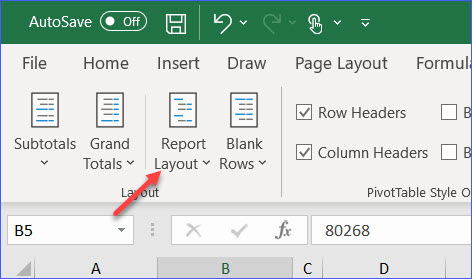
How to Change Pivot Table in Tabular Form - ExcelNotes

Excel Help: Simple method to make Pivot table

How to make row labels on same line in pivot table?
Classic PivotTable Default Layout • My Online Training Hub
How to Change Pivot Table in Tabular Form - ExcelNotes

How to Sort Pivot Table Row Labels, Column Field Labels and Data Values with Excel VBA Macro ...
Post a Comment for "42 pivot table 2 row labels"